Ex 4.2: Threshold-based tissue segmentation	•	Ex 4.4: Semi-automatic segmentation using SAM

4. Tissue segmentation and classification

4.3 Using a N-classes pixel classifier

In the last exercise, we discovered a simple way to extract our objects using a simple thresholder, but they are very limited in terms of what they can see (only based on intensity) and we are limited to two classes (true/false, +/-, FG/BG, ...)

We would like to have a way to segment areas in our tissue based on features more subtle than just the intensity. We would also like to have the possibility to classify more than two types of tissue.

Note

Don't forget to create a new project for this exercise and keep it tidy, we will use it again in another exercise.

4.3.1 Epithelium area in colorectal cancer

Goals:

• The goal of this exercise is to measure the area of epithelium in images of colorectal cancers.
• To do so, you will need to:
  • Find the polygon corresponding to the whole tissue and give it the Colon classification using a thresholder.
  • Make a training image from a set of representative chunks of image.
  • Train a pixel classifier able to differentiate the epithelium from the rest of the tissue.
  • Apply the pixel classifier to find epithelium detections within the colon annotations.
  • Export the measurements to a TSV.

Required data:

Folder	Description	Location	License
Colorectal Cancer IHC HE	Whole slide images of colorectal cancer stained with hematoxylin and eosin	DOI: 10.18710/DIGQGQ	CC0 1.0

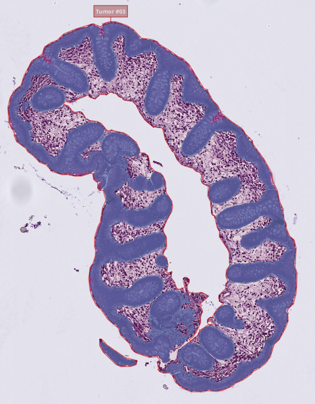
A. Locate the tissue on the slides

• Before starting this step, make sure that you have the Tumor class available in your class list. It is part of the built-in classes of QuPath so it should already be present for everybody.
• Using the protocol described in Ex 2: Threshold-based tissue segmentation, create the threshold classifier segmenting the tissue on your slides. Make sure that you split objects into separate polygons so you can filter the polygons by area and give a name to the different parts so you can find in the final TSV which line corresponds to which object.
• Using the workflow recorder, apply the thresholder to all the images of your dataset and clean up the results where it's required:
  • Remove the undesired parts (bubbles, folded tissue, ...)
  • Merge fragmented tissue into unique polygons
  • Give a name to each chunk to recognize them later (In the annotation list: right-click > Set properties > Name)
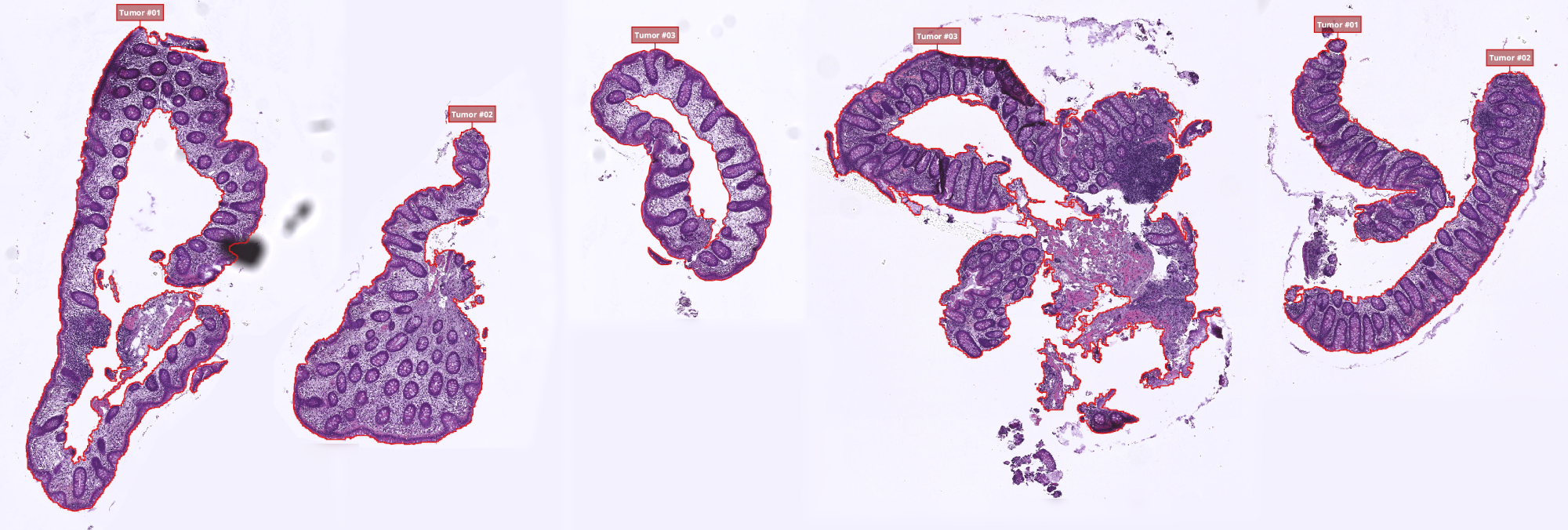
• At this point, each image that you have should contain several polygons classified as Tumor.
• If you gave names to your annotations but they don't show up in the viewer, try to click on the "toggle names display" button.

B. Create a training image

• The pixel classifier that we will use later is based on a machine learning algorithm, so we need to show it a representative sample of data.
• We can't simply search through our whole project and hope to find an image representative of the entire dataset.
• To address this need, we will create a new image being a patchwork of representative chunks selected throughout our project.
• In order to do that, make a checklist of the different textures that you can find your your images, for example:
  • Where the nuclei are very dense
  • Where there is almost no nuclei
  • Where you have small/huge crypts
  • Where the staining is lighter/darker than usual
  • ...
• Once you identified all the textures, for each of these textures:
  • Find an example of area where this texture is present
  • Activate your rectangle selection tool and make a rectangle around this example
  • Give the Region* class to this newly created rectangle

Note

Don't forget to include a couple of normal/clean areas in your Region* rectangles, it would be a shame if the classifier only behaved well on unusual cases!

• Once you made a few rectangles containing examples over your images, we will use them to create our training image summarizing most of what we can find in our dataset.
• To do that:
  • Save your project.
  • In the top-bar menu, go to: "Classify" > "Training images" > "Create training image...".
  • If you used the Region* class for your example rectangles, you don't have to edit the settings, you can just validate.
  • In your list of images, a new "Sparse image" should have appeared.

Note

Don't forget to do the color deconvolution for all the images of this project, including the training image ("Sparse image")!!!

C. Train the pixel classifier

• In QuPath, training a pixel classifier based on machine learning (K-nn, random forest, ...) is an iterative process. It means that we will start by providing it with a very few examples and see what it understands. According to its errors, we will add a few more examples and see how it helps it. We do that as many times as it takes to get a descent result.

Note

For pixel classification, examples can be provided using any selection tool and any type of annotation. Despite that, we make the general assumption that in an image, two pixels located side by side (or very close from one another) carry very similar information. Based on that, we usually restraint ourselves to point selections to provide examples. It makes it easier to see what the classifier uses by the end, and makes the training phase faster as the number of pixels to process is kept under control.

Also keep in mind that QuPath represents points by a little circle, but it is just for visualization. Points are a (x, y) coordinate, they don't have any area: the pixels enclosed in the circle don't matter, only the one under the very center of the circle does.

a. Place your first set of examples

• It is now time to start our first iteration of the training process by creating our first set of examples.
• Before starting, make sure that you have the Epithelium, Other and Ignore* classes in your classes list.
• In the following instructions, we will use point annotations to make our examples, but feel free to experiment any type of annotation. You can mix all types of annotations if you wish.
• Go to your "Sparse image" and click on the point annotation tool. You should now see a new floating window allowing to create/edit point annotations.
• In this exercise, we will try to isolate:
  • the epythelium (including the crypts) (as Epithelium)
  • the regular tissue (as Other)
  • the enclosed background (as Ignore*)
• We don't have to take care of the non-enclosed background because we already eliminated it with our thresholder.
• In the floating window, you can click on "Add" three times (once for each item enumerated above). Each time you click, a new empty points cloud should appear in the list just above the "Add" button.
• Click on the first points cloud in the list, then on the Epithelium class, and bind them using "Set selected". Repeat this operation with the second points cloud and Other, as well as the third and Ignore*. If you did things correctly, the icon of each points cloud should now have the color of the class you bound it with, and the name of the class should be indicated next to it.
• Starting with the epithelium+crypt tissue, we will provide a few examples:
  • Limit yourself to 20 to 30 examples.
  • Place some points on all your patches.
  • Save often.
  • Don't place points close to the connection between two patches.
  • Don't place points next to the black background.
  • Place some points at the boundaries of each areas.
• Repeat this step for the regular tissue and the enclosed background.
• Save your project.

Warning

During the training process, reprocessing everything is a rather heavy process causing QuPath to crash very often. Saving your project after placing points, removing points, tweaking settings, ... should be a reflex.

b. Instanciate the pixel classifier

• In the top bar menu, go to "Classify" > "Pixel classification" > "Train pixel classifier...".
• A new floating window should appear with everything you need to configure our new pixel classifier.
• You can start by settings the classification algorithm to "Random trees", other algorithms are not robust enough for what we are going to do (you are free to try them out though, the instructions don't change).
• We are looking for huge objects: nothing depending on a very fine texture or filaments, so can limit our working resolution to "Moderate" or "High".

Tip

In the step described below, we will use the "Live prediction" that keeps reprocessing everything everytime you edit the settings or modify your examples. If you have a "modest" computer, zoom a lot before activating it to avoid refreshing the whole image at once and crashing QuPath.

c. Choose the features and the radii

• To determine what's present on a pixel, the classifier builds a vector (collection of numbers).
• To process the values contained in this vector, N filters (Gaussian, Weighted magnitude, ...) are applied at M different radii (2, 4, 8, ...) for your C channels. The vector contains CxMxN values. Such vector is processed for every single example pixel you provided.
• As you may expect, it is a heavy task, so we will try to avoid asking for useless filters and/or useless radii. The goal is to only keep the filters and radii that highlight what we are interested in.
• To start, you can:
  • Click on the "Edit" button at the Classifier line and activate the "Calculate variable importance".
  • Open the features list by clicking on the "Edit" button at the Features line, and only take the Hematoxylin and Eosin channels.
  • Activate the "Live prediction" to see in real time the effect of what you do.
• Now, we will iteratively choose our filters and radii:
  • Open the features list by clicking on the "Edit" button at the "Features" line.
  • In the "Scale", try to add/remove a few neighborings radii (whichever you want, but don't go higher than 12 included if you don't want to kill your PC)
  • In the "Features", try to add/remove some filters (whichever you want)
  • Click the "OK" button (that should close the "Select features" window)
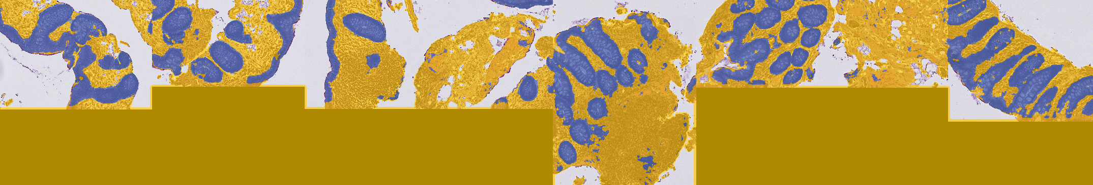
  • In the lower right corner of the "Train pixel classifier" window, you should have a dropdown menu containing "Show classification" for now. Click on it. It contains the result of every filter for every channel for all radii.
  • For a same filter, look at all the channels and all the radii. If the result is plain gray all the time (in the main viewer), it means that this filter is useless, you can remove it.
  • If the result is plain gray only for some radii, remove these radii from your list.
  • If everything present on the slide is highlighted or if the result is chaotic, the filter is just as useless as if it was plain gray, you can remove it (see examples below).

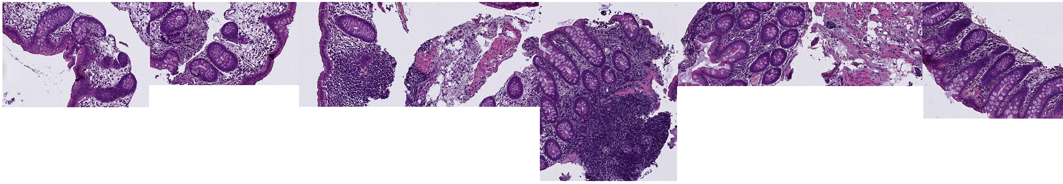
Original image	Empty / chaotic	Interesting

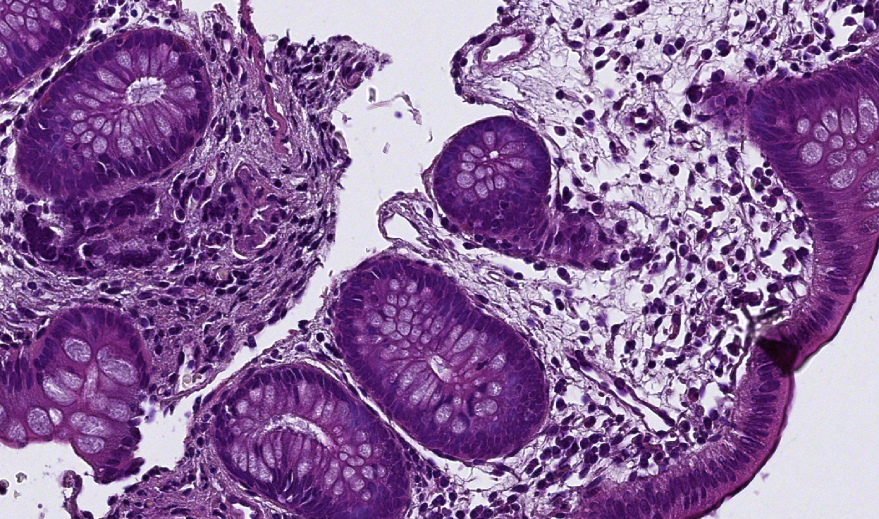• If you struggle finding your features and your radii, you can try with the following settings (they should be a descent starting point):
  • Resolution: "High"
  • Features window:
    • Channels: "Hematoxylin", "Eosin"
    • Scales: 4.0, 8.0, 12.0
    • Features: Gaussian, Laplacian of Gaussian, Weighted deviation, Gradient magnitude

d. Refine the classification

• You are now done with choosing your filters and your radii, it is time to add more examples to refine the classification.
• Make sure that the dropdown menu is back to "Show classification"
• Look where your classifier made mistakes and add a point there.
• You can use the "toggle classification" button to show/hide the preview or use the slider beside it to make it semi-transparent.
• Try to keep the number of points for each class approximately in the same range.
• Every time you notice an improvement:
  • Save your project
  • Save your classifier by giving it a name and clicking "Save" (in the "Train pixel classifier" window)
• Once you are satisfied with the result, save the classifier a last time, save your project, and you can now close the "Train pixel classifier" window.

D. Apply the classifier

We successfully made a pixel classifier able to tell for each pixel of our image whether it's nothing, regular tissue or epithelium. Now, we need to tell QuPath to use this classifier only in the Tumor annotations that we found earlier and to create polygons around each island of tissue and epithelium. We will then remove polygons of regular tissue as we are not really interested in them. Eventually, we will make a script to apply that to our whole project.

a. For one image

• Start by opening any of the images containing some Tumor polygons.
• If some Region* annotations are present on this image, do a right-click on Region*in the class list and "Select objects by classification". You can then click on "Delete", below the annotation list.
• Again, do a right-click but on Tumor this time and "Select objects by classification" (don't delete them this time).
• In the top bar menu, go to "Classify" > "Pixel classification" > "Load pixel classifier...".
• In the "Choose model" dropdown of the floating window, select the pixel classifier that we just trained.
• If you click of "Create objects", QuPath will ask you where to create the objects. We want to make them in the Tumor polygons that we just selected, so we should set the parent object to "Current selection", and press "OK".
• In the new window that appeared, we will set the object type to "Detection" (we don't need to edit the epithelium objects about to be found, so we don't need annotations). If your classifier has a tendancy to generate small debris or holes, you can try to augment the "Minimum object size" and "Minimum hole size". You don't need to change any other setting, you can just validate.
• QuPath will freeze for a few second, the time to process the new polygons.
• Once you can interact with QuPath again, the "Load pixel classifier" window should still be opened. Click on "Add measurement". Again, make sure that "Select objects" is set to "Current selection" to measure inside our Tumor annotations.
• You can validate, save your project and close the floating window.
• As mentionned previously, we are not really interested in the regular tissue (to which we gave the Other class). So you can do a right-click on Other, "Select objects by classification" and "Delete".
• You should be left with your Tumor annotations containing an Epithelium polygon.
• If you go in the "Hierarchy" tab (next to the "Project", "Image", "Annotation", ... tabs), you will be shown which polygon is parent of which. At first, you should only see your Tumor annotations, but if you unfold them, you should see the Epithelium detection within them.
• If you click on any Tumor annotation, you should see in its properties (lower left panel of QuPath) some lines starting with the name of your classifier and some associated measurements.

b. For the project

• In this step, we will reproduce the same step, but using QuPath's scripting language.
• Start by going to the "Workflow" tab, and convert your history of commands to a script using the "Create script" button.
• To avoid working in the mess of the commands history, in the script editor, go to "File" > "New" to create an empty file. Your can navigate between bot hyour script using the left column of the script editor.
• The first thing that we did was to select and remove the Region* annotations.
• In the history, you should find the two lines to select objects by the Region* classification and remove selected objects. Copy them into your clean script.
• If you want to write some notes for later in your script, you can turn any line into a comment by making it start with "//".
• Then we selected our Tumor annotations to run the classifier only in them. Copy the line to select objects by Tumor classification into your clean script.
• After that, we launched our classifier to create the detection. Find and copy the line that creates detections using your classifier into the clean script.
• To have an area in µm², we added a measurement using our classifier. You can transfer this line in the clean script as well.
• Eventually, we selected and removed the Other objects, so you can find and copy the lines to select objects by Other classification and remove them.
• You should be left with a script looking like that:

// Remove the `Region*` annotations that we made for training
selectObjectsByClassification("Region*");
removeSelectedObjects()

// Select the tumor annotations found earlier
selectObjectsByClassification("Tumor");

// Make the `Epithelium` and `Other` detections using the "find-epithelium" classifier
createDetectionsFromPixelClassifier("find-epithelium", 1000.0, 1000.0);

// Measure the areas of epithelium
addPixelClassifierMeasurements("find-epithelium", "find-epithelium");

// Select and remove the non-epithelium areas
selectObjectsByClassification("Other");
removeSelectedObjects()

• Save this new script into your project (QuPath will suggest you a location, keep it. Just provide a name).
• Use the "more options" button next to the "Run" button, and choose "Run for project".
• Transfer all the images to the right except for the image on which we made the process manually, and the sparse image.
• Launch the process. Once it is done, save your project before doing anything.
• You can navigate in the images of your poject to see the results.

E. Export the measurements

• Start by saving your project.
• You can now go to "Measure" > "Export measurements...".
• Transfer your images to the right column (except for the "Sparse image").
• Provide a path for the TSV that will contain the results.
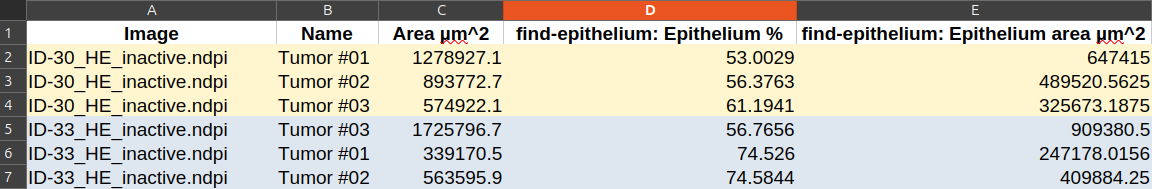
• The information of area that we area interested in is stored in the annotations.
• If you export the measure, open them in a spread sheet and remove the useless columns, you should be left with something looking like that: