3. Stain Separation by Color Deconvolution

In fluorescence microscopy the channels of different light emitting fluophores are registered independently. As long as the are channels acquired correctly, it is clear what the value of each channel for a given pixel is. For brightfield images with histochemical stainings the situation is different. In this case the red, green and blue components of the light not blocked by the stainings is registered and it is not clear what the participation of each stainig to the resulting value is. This can to some degree be helped using color deconvolution.

3.1 Fluorescence vs. Brightfield Microscopy

Fluorescence microscopy works by exciting a fluophore, using light of a specific wavelength, which results in the fluophore emitting light of a different specific wavelength, which passes a filter and is captured by a monochrome camera as a grayscale image. Multiple fluophores can be used to acquire images of multiple channels which can be assembled to a composite image.

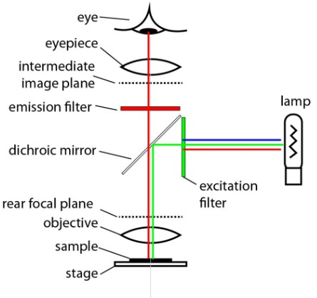
Fig. 3.1 – Schema of an epifluorescence microscope.

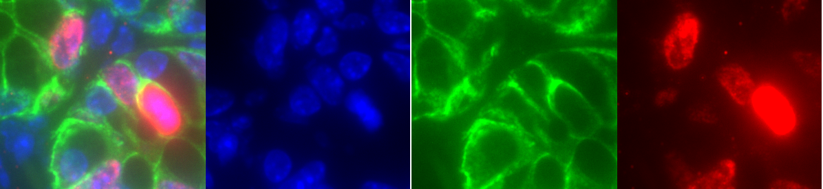
Fig. 3.2 – Composite image and the individual channels.

In brightfield microscopy, the transmitted light, i.e. the light that is not absorbed is recorded using an RGB-color camera. The participation of each staining, for example hematoxilin and eosin, to the red, green and blue components of a pixel is not clear.

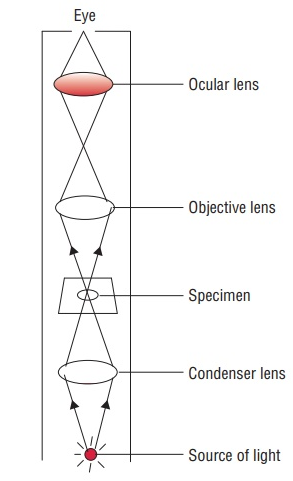
Fig. 3.3 – Schema of a compound microscope [2].

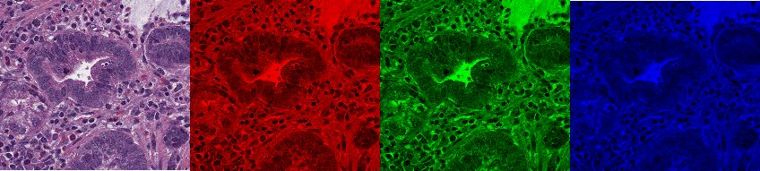
Fig. 3.4 – RGB brightfield image and its red, green and blue channels.

3.2 Color Deconvolution

The objective of color deconvolution is to calculate the contribution of each of the stains based on the stain specific RGB absorption. Color deconvolution has been proposed in 2001 by Ruifrok and Johnston [1].

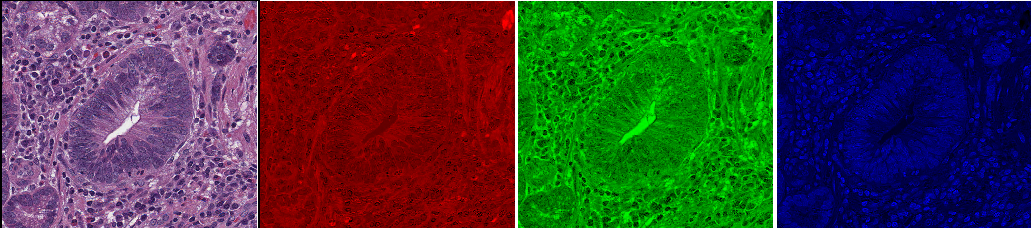
Fig. 3.5 – The rgb image with the red, green and blue channels.

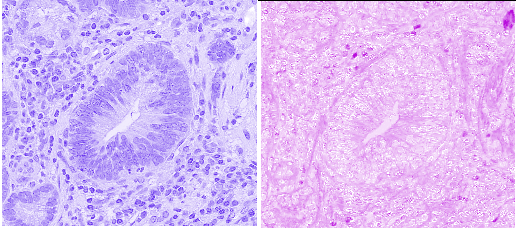
Fig. 3.6 – The channels of the hematoxylin and eosion contributions.

3.2.1 Lambert-Beer's Law

The transmitted light $I_c$ in a channel $c$ (red, green or blue), depends on the entering light intensity in the channel $I_{0,c}$, the amount of stain $A$ and the absorption factor of the stain in the channel $c_c$

$$ I_c = I_{0, c} \cdot e^{-A \cdot c_c} \tag{3-1} $$

The relation between the intensity in the image and the amount of stain is not linear. But the optical density is linear in the amount of stain for each channel.

$$ OD_c = -\log_{10}\left(\frac{I_c}{I_{0,c}}\right) = A \cdot c_c \tag{3-2} $$

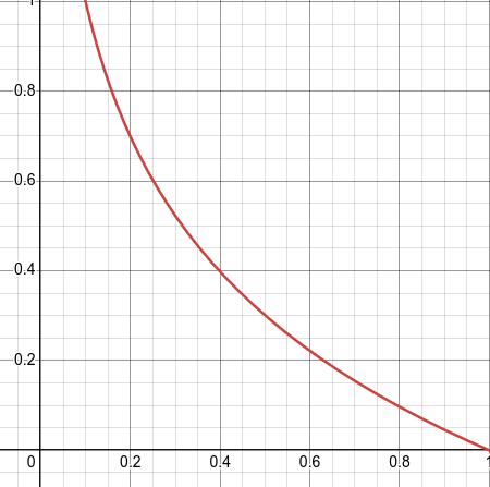
Fig. 3.7 – Optical density for the ratios of transmitted to entering light between O and 1.

3.2.2 The optical density and the deconvolution matrix

Each pure stain (hematoxylin, eosin, ...) has a specific optical density RGB-vector. These vectors form the rows of the optical density matrix.

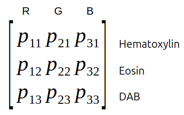
Fig. 3.8 – The optical density matrix.

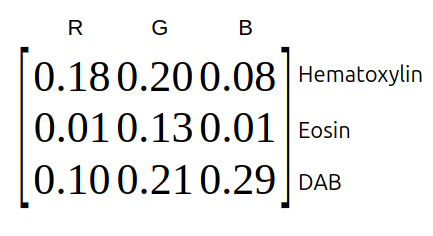
Fig. 3.9 – Example of an optical density matrix.

We normalize the optical density matrix by dividing each component by the length of its row vector and calculate the inverse matrix of the result. This matrix is called the deconvolution matrix $D$. If we multiply the deconvolution matrix with the optical density vectors of the image, we obtain an orthogonal representation of the stains forming the image.

Note

To normalize the value $p_{11}$ calculate:

$$ \sqrt{p_{11}^2 + p_{21}^2 + p_{31}^2} \tag{3-3} $$

The inverse matrix $A^{-1}$ of the matrix $A$ is a matrix so that:

$$ A \cdot A^{-1} = I \tag{3-4} $$

where $I$ is the identity matrix that has the value one in the diagonal and zero everywhere else.

3.2.3 Color Deconvolution in QuPath

To apply a color deconvolution, we need to calculate the optical density values of the image. To do that, we need to know the entering light intensity in each channel $I_{0,c}$. We assume it to be the value of the channel in a background region, since the background is empty and should let pass all of the incoming light.

We also need to know the OD-RGB vectors of the pure stains in the image. There are three approaches:

1. Use predefined standard values for each stain
2. Measeure the values from locations of pure stain in the image (Ideally you should have single stained slides for this)
3. Auto-estimate them from the distribution of the RGB values

Predefined values are applied when the image type is set to Brightfield H&E, Brightfield H-Dab or Brightfield other. You can see and modify the values on the image-tab. A double-click into the value field of the background or one of the stain values, lets you manually set the vectors. You can check the result via the brightness and contrast tool or via the channel viewer. When the image only contains two stains the third channel contains the residuals.

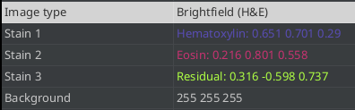
Fig. 3.10 – The background and stain vectors on the image tab.

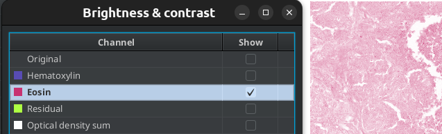
Fig. 3.11 – Using the B&C tool to display the result of the color deconvolution.

If you have a selected annotation when you double click the background or stain value, the vectors will be set from the values in the roi for each rgb-channel.

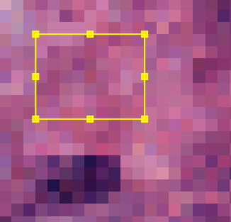
Fig. 3.12 – Setting a stain vector from a ROI.

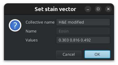
Fig. 3.13 – The values have been taken from the ROI.

You can let QuPath automatically estimate the stain vectors. It uses a variation of the method introduced in [2]. To use this method select a region that contains the different stainings and some background. When you run the command Estimate stain vectors... from the menu Analyze QuPath will first find the most common background value in the region and propose to use it. If you have set the correct background value before and you want to keep it, you can answer with no. The visual stain editor will then be opened.

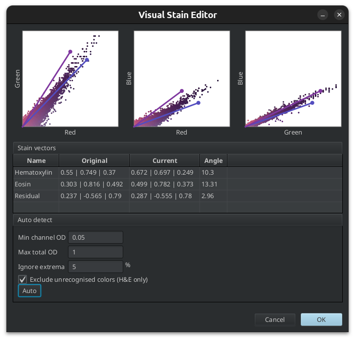
Fig. 3.14 – The visual stain editor.

The parameters allow to ignore very low optical density values for each channel. These correspond to regions with very little stain. [2] proposes a value of 0.15 for this. The maximum total optical density can also be restricted, excluding very dark regions from the analysis. Finally a percentile can be set to ignore extreme values which might be outliers.

You can apply the background and the stain vectors to multiple images using a script. The colors and the background of the images must be sufficiently similar of course.

Set the values on one image, then go to the Workflow-tab and press the Create script...-button.

Script 3.1 – Set the stain vectors and the background vector.

setImageType('BRIGHTFIELD_H_E')
setColorDeconvolutionStains('{"Name" : "H&E modified",\
                              "Stain 1" : "Hematoxylin",\ 
                              "Values 1" : "0.589868825130324 0.6695953191368946 0.45132790488660385",\
                              "Stain 2" : "Eosin",\
                              "Values 2" : "0.39491445806317216 0.7836975302156244 0.47943795421994034",\
                              "Background" : " 243 239 239"}');

Run the script on multiple images, using the command Run for project from the script editor's Run-menu.

3.2.4 Limits

With RGB images color deconvolution can be used to separate 2 or 3 stains, not more. It's main utility is to facilitate the segmentation of cells and other structures and to classify them into a small number of classes, for example positive and negative. However it can not be interpreted quantitatively. For DAB-staining the case is worse, since it scatters light rather than absorbing it. It does not follow the Beer-Lambert law.

Literature

1. Ruifrok, A C, and D A Johnston. Quantification of Histochemical Staining by Color Deconvolution. Analytical and Quantitative Cytology and Histology, 23 (4): 291–9, 2001.

2. Macenko, M., Niethammer, M., Marron, J.S., Borland, D., Woosley, J.T., Xiaojun Guan, Schmitt, C., Thomas, N.E., 2009. A method for normalizing histology slides for quantitative analysis, in: 2009 IEEE International Symposium on Biomedical Imaging: From Nano to Macro. Presented at the 2009 IEEE International Symposium on Biomedical Imaging: From Nano to Macro (ISBI), IEEE, Boston, MA, USA, pp. 1107–1110.

References

1. The epi-fluorescence microscope from https://bookdown.org/jcog196013/BS2010_Notes/wide-field-microscopy.html

2. The compound light microscope from https://www.brainkart.com/article/Light-microscopy_17818/