2. Navigation, Annotations and Measurements

In order to efficiently use QuPath in your image analysis projectcs, you need to understand its basic tools first. In this chapter you will first see how to navigate within an image and how to change the contrast settings. You will then learn to use the different types of annotation tools and how to configure, make and export shape and intensity measurements.

2.1 Navigation

2.1.1 The image viewer

Double click the thumbnail of an image to open it in the image viewer.

In the upper left corner you find the overview window of the image. It situates the current view in the image, if the view shows less than the whole image. You can click into it to move the view to a location. In the lower right corner you find the coordinates of the mouse pointer and the intensity value of each channel. In the lower left corner a scalebar is displayed. You can show and hide these elements from the View-menu.

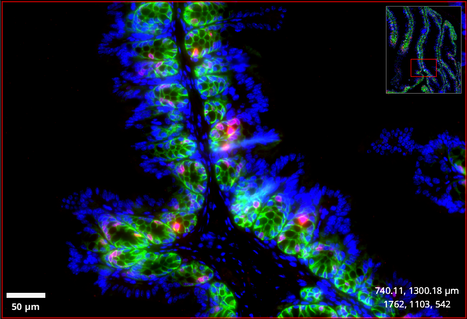
Fig. 2.1 – QuPath's image viewer with overview, coordinates/intensities and scalebar.

To navigate within the image use:

Zoom

+ +

Pan / Shift

When move tool selected:

+

When annotation tool selected:

+ +

You can also set the view to some predefined values from the Display-submenu of the image viewer's context menu. The View>Zoom-menu of QuPath offers another possibility to modify the zoom. On the toolbar you find the button , that sets the zoom, so that the image fits into the window and a button showing the current zoom , that you can double-click to enter an arbitrary zoom factor.

2.1.2 Adjust Brightness and Contrast

Depending on the intensities in the image, you might need to adjust the brightness and contrast of the different channels of an image. Press the button or use the keyboard-shortcut + to open the Brigthness and Contrast Tool (B&C).

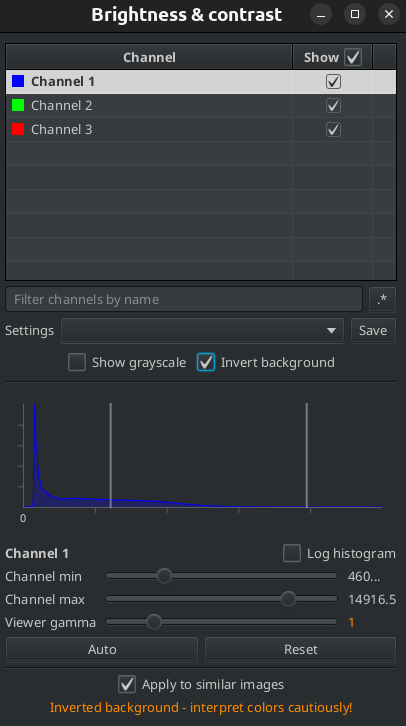
Fig. 2.2 – The Brightness and Contrast Tool of QuPath.

The upper part lists the channels of the image. You can select for channel if it is displayed or not. This can also be achieved via the keyboard-shortcuts , , , etc., without opening the B&C-tool. A double-click on the name of the channel allows to change its name and its color. If you select Show grayscale only the channel currently selected channel is displayed as a grayscale image.

The middle-part shows the histogram of the selected channel. On the x-axis are the intensities in the image, segmented into bins of the same size. On the y-axis is the number of times each intensity or the intensities in each bin are present in the image. The two horizontal bars represent the minimum and maximum display value. Intensity values in the image below the minimum display value will be displayed as 0 and values above the maximum as the maximal value possible. Values between will be mapped linearly using the line defined by the points (min-display-value, 0) and (max-display-value, max-possible-value). You can change the brightness and contrast of the display of a channel using the Channel min and Channel max sliders. Reset will set the minimum display value to zero and the maximum display value to the maximum intensity value in the channel. The Auto-button will find minimum and maximum display values automatically, based on the histogram of the image.

If you invert the contrast or use the non-linear gamma-display-adjustment, QuPath will emit a warning to make sure that the displayed intensities will not be misinterpreted.

You can save the display settings and apply them to other images. For this to work all images must have the same number of channels with the same names.

2.1.3 The Image-Tab

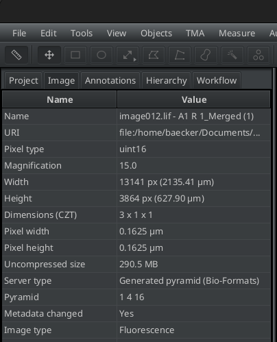
Fig. 2.3 – The image-tab displays informations about the image and allows to modify some of the metadata.

Under Pyramid you can find the down-scaling factors of the image pyramid. The values that can be modified by double-clicking into the value-cell are:

• the magnification of the full resolution
• the pixel size
• the image type

For brightfield images you will also be able to modify the stain vector for each channel and the vector for the background. You will learn more about this in the chapter Color Deconvolution.

You can reset the changes you made via the value of Metadata changed.

2.1.4 The Multi-View

The multi-view allows to open more than one image at the same time.

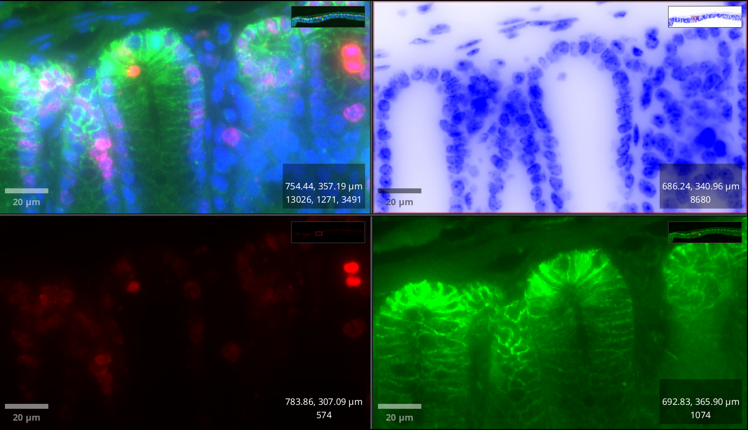
Fig. 2.4 – Four versions of the same image in the multi-view.

From the context-menu of the image-viewer you can set the grid-size of the multi-view. Clicking into a cell activates it. When you open an image it will be opened in the active cell.

You can also use the multi-view to display and synchronize multiple views of the same image. In order to do this, you must first make duplicates of the image. Open each duplicate in its own viewer and use the Brightness and Contrast-tool to show a different channels in 3 of the views. Use Multi-view>Synchronize viewers to synchronize the views.

Note

Make sure the option Apply to similar images on the B&C is not selected, otherwise hiding and displaying channels will affect the open images in all views.

2.2 Annotations

Annotations are an important tool in QuPath. Whenever you run an operation, for example cell detection you need to specify one or more annotations on which the operation will work. Annotations can also be used for the communication between humans. A pathologist can for example annotate a zone of anormal tissue and attach a name and a description containing his observations and a diagnosis.

Annotations can be 2D areas, lines or points. A class can be attributed to an annotation, manually or by running a machine learning object classifier. The shape and intensity features of a zone specified by an annotation can be measured. Examples of possible measurements are:

• area
• perimeter
• diameter
• length
• number of objects within
• intensities in the different channels

Annotations can be used as selections, for example to select regions of interest for further analysis or to reduce an operation to a small zone while still adjusting its parameters. Annotations can also be the result of an operation, for example when running a pixel classifier for tissue segmentation.

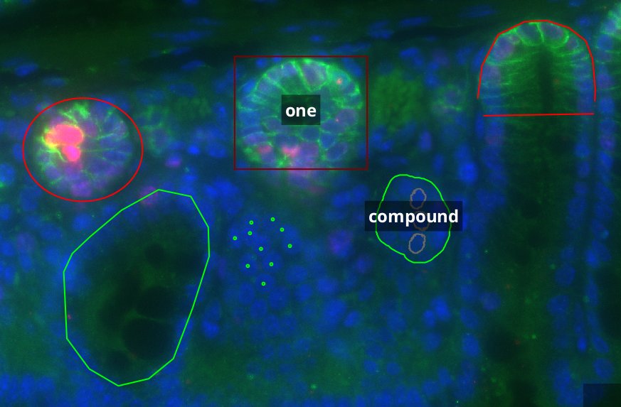
Fig. 2.5 – Different kinds of annotations.

2.2.1 Annotation Tools

The tools for annotating areas are: Rectangle, Ellipse, Polygon, Brush and the Magic Wand. When the tool is selected and you click into the image and move the mouse, you are creating the an annotation. You can restrict the rectangle to a square and the ellipse to a circle, by pressing when creating the annotation. The brush tool allows to paint area annotations with a brush. The wand tool is like the brush tool, but stops automatically when the intensity values differ too much from those of the pixels in the area clicked on in the beginning. To remove parts from an annotation with the brush or wand tool hold down while using the tool. Note that the granularity of the brush and wand depend on the zoom. Zoom-in to select finer details and zoom-out to select larger areas more quickly.

The tools for line segments are Line and Polyline. To create a polygon or polyline, you move the mouse and click for every point you want to add. Double-click to finish the annotation creation. Instead of line segments, you can also select to use arrows from the menu button of the line tool.

Points are used to count objects or to select objects for the training of an object classifier.

Fig. 2.6 – The annotations toolbar.

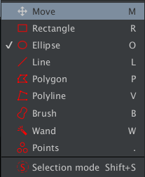
Fig. 2.7 – The tools menu.

Each time you finish an annotation, the annotation tool is unselected and the Move tool is selected instead, so that you can move to another location. It is therefore useful to remember the keyboard shortcuts for selecting the annotation tools, see Fig. 2.7.

When you select the point tool a window is opened, which allows you to create point sets. The tool then adds the points to the active point set. Note that for the point-tool the tool is not deselected after making a point. To navigate to a location while the point tool is active, hold down space and drag the image.

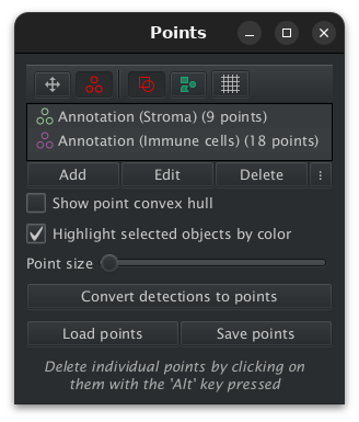
Fig. 2.8 – The window of the points tool.

2.2.2 The Annotations Tab

The annotations tab allows to select and manipultae annotations. It consists of the annotation list, the class list and an area displaying either the measurements of the selected annotation or its description.

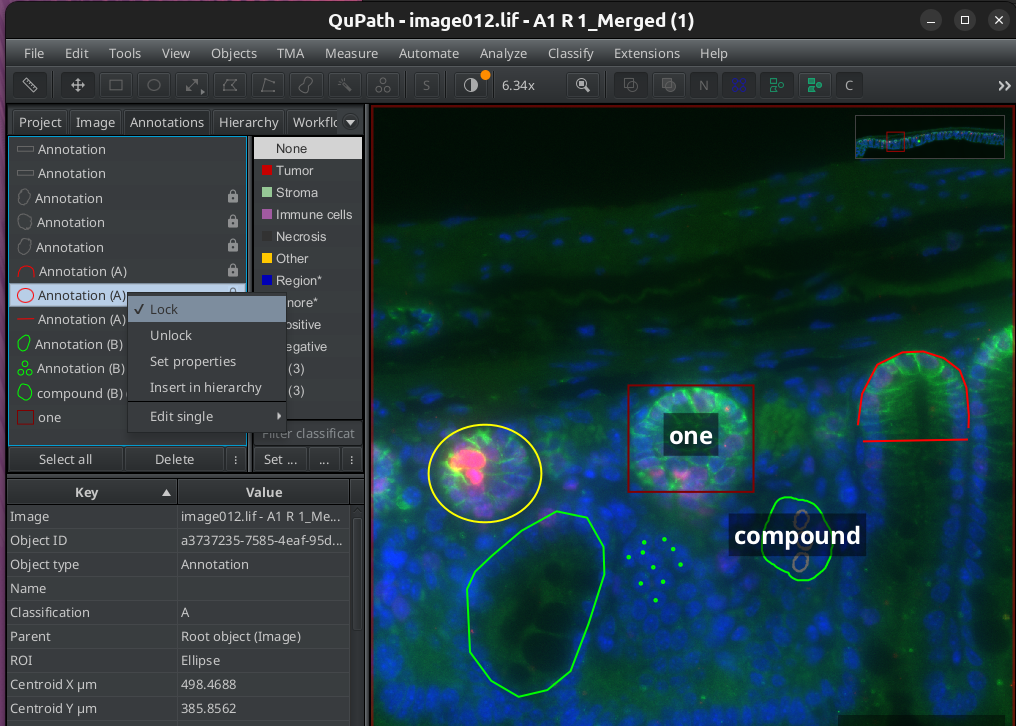
Fig. 2.9 – The annotations tab.

In the annotation list you can select one or more annotations. If you click on a single annotation it will be selected. If you double-click it, it will be selected and the view will be changed to show it in the middle of the viewer. To select multiple selections, use shift or ctrl. You can lock annotations from the context menu of the annotation list. Locked annotations can only be modified after they are unlocked again. When running operations you can choose to run them on locked annotations. If you select an annotation in the image, by double-clicking it, it will also be selected in the annotation list.

2.2.3 Selecting Annotations in the Image

On the image you can select and delete annotations using:

Select all annotations

+ +

Do not confuse with make a new annotation of the whole image

+ +

Add or remove an annotation from a selection

+

Delete the selected annotations

or

You can also use the Delete objects command that you can find in the viewer's context menu, when one or more annotations are selected.

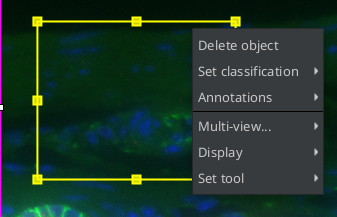
Fig. 2.10 – Deleting objects from the viewer's context menu.

2.2.4 The Selection Mode

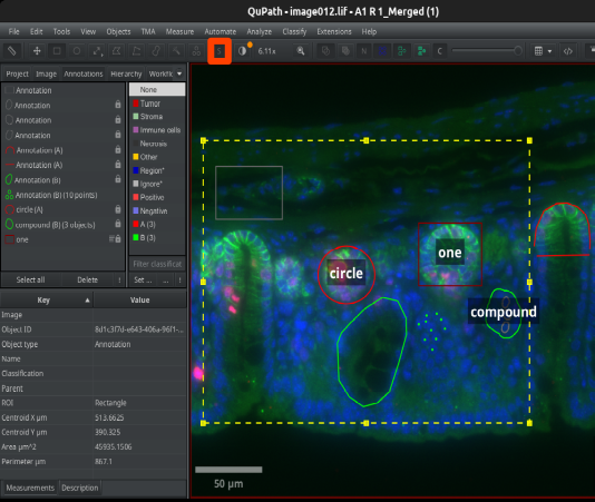
Fig. 2.11 – In Selection Mode the annotation tools select annotations instead of creating them.

In Selection Mode you can use the annotation tools to select annotations. Toggle the Selection Mode by pressing the button . By pressing you can add annotations to an existing selection and by pressing you can remove them from it.

2.2.5 Annotation Properties

You can modify the properties of one or multiple selected annotations via the command Set properties from the submenu Annotations of the viewer's context menu or from the context menu of the Annotation list.

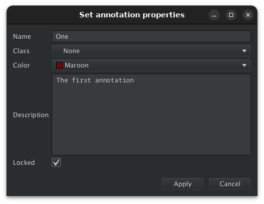
Fig. 2.12 – Modifying the properties of annotations.

The properties of an annotation are: its name, its class, its color, its description and whether it is locked or not. When you attribute a class to an annotation the annotation's color will be set to the color of the class and the Color-input will be ignored. When you modify the properties of an annotation, that already has a class and you do not change the class, the annotation's color will be the one selected in the Color-input field.

2.2.6 Editing Annotations

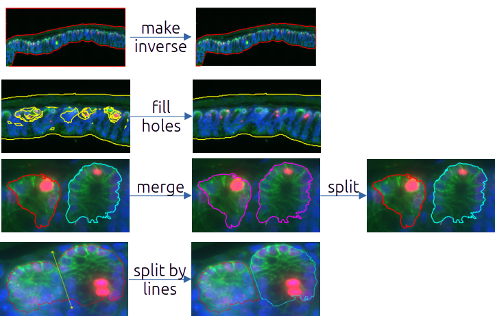
Fig. 2.13 – Some of the operations on annotations.

You can find the operations on annotations in the Annotations context menu and in the menu Objects>Annotations.

Operations to create an annotation:

• create full image annotation -- Objects>Annotations>Create full image annotation... -- + +
  • Create an annotation that contains the whole image. Some operations need a root object, the full image annotation can be used if the operation should be applied to the whole image.
• specify -- Objects>Annotations>Specify annotation...
  • Create a new Rectangle or Ellipse annotation, by specifying its width and height and its coordinates.

Operations on one annotation:

• copy to current plane -- Objects>Annotations>Copy annotations to current plane -- + + This command assumes that you are working on a time series or z-stack. The selected annotations will be copied to the currently selected plane.
• duplicate -- Objects>Annotations>Duplicate selected annotations -- +
  • Duplicates the selected annotations.
• expand -- Objects>Annotations>Expand annotations
  • Enlargen an annotation by a given radius. To create a band of radius r around the border of an annotation: Expand the annotation by r, then select the option Remove interior and expand the resulting annotaion by -2r.
• fill holes -- Objects>Annotations>Fill holes
  • Fill the holes in the annotation. Areas completely surrounded by the annotation will become part of the annotation.
• make inverse -- Objects>Annotations>Make inverse
  • Add an annotation that contains the parts of the image not contained in the selected.
• simplify shape -- Objects>Annotations>Simplify Shape..
  • An annotation that has been created with the polygon, brush or wand tool might have too many vertices defining its border. This can also be the case when the annotation is the result of an operation. All these fine details on the border will arbitrarily augment the perimeter measurement. This operation simplifies the annotation by removing unnecessary vertices while trying to keep the same shape.
• split -- Objects>Annotations>Split annotations
  • The unconnected parts of the annotations will become an annotation each.
• transfer -- Objects>Annotations>Transfer last annotation -- +
  • Transfer the last selected annotation from one image to another. You need to be in a new image when runnning the command, either using the grid view, or after having closed the first and opend the second image.
• transform -- Objects>Annotations>Split annotations -- + +
  • A round handle will appear above the annotation. Grab the handle and rotate the annotation by moving the mouse.

Operations on at least two annnotations:

• intersect -- Viewer's context menu>Annotations>Edit multiple annotations>Intersect selected
  • Replace the selected annotations by their intersection. The result is the zone in which all participating annotations are overlapping. If there is one annotation that does not overlap with the overlapping zone of all others, the intersection is empty and as a result the participating annotations are removed.
• merge -- Objects>Annotations>Merge selected
  • Merge the selected annotations. The result is an annotation formed of the union of the annotations.
• subtract -- Viewer's context menu>Annotations>Edit multiple annotations>Subtract selected
  • Subtracts all the selected annotations from the one selected last. Note that only the subtracted area remains, the annotations subtracted from the last one will be removed.

Others:

• Split by lines -- Objects>Annotations>Split annotations by lines...
  • Splits single annotations into multiple annotations using all line or polyline annotations crossing the single annotations.
• Remove fragments and holes -- Objects>Annotations>Remove fragments & holes
  • Removes small fragments in the background and small holes in the annotations. This is often usefull to clean up, after an instance segmentation, for example with a pixel classifier, has been done. When applying a pixel classifier to create objects, there is an option, that already applies this operation.

2.2.7 The Annotation Hierarchy

If you want to count or analyze objects included into other objects, you need to take into accoount the hiearchy of the objects. You could for example have multiple sections on each slide and within each section multiple tissue regions of interest, each one containing the objects of interest. QuPath can represent hierachical relationships, using a hierachy of annotations. To be considered a sub-annotation of a parent-annotation, the annotation must be completly within the parent-annotation. You can either insert single annotations into the hierachy or let QuPath automatically resolve the whole hiearachy for all annotations. The hierachy-tab allows to select the annotations from the hierachy-tree using a mouse click and to select and display them using a double-click, the same way as on the annotations-tab.

• insert into hierachy -- Objects>Annotations>Insert into hierachy -- + +

  • Inserts the selected annotations into the hierachy.

• resolve hierachy -- Objects>Annotations>Resolve hierachy -- + +

  • Resolves the included in-hierachy for all annotations.

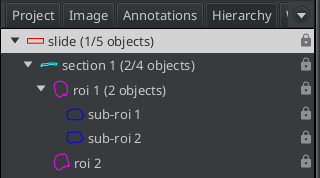
Fig. 2.14 – The tree of annotations on the hierachy-tab.

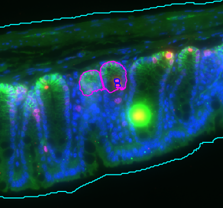
Fig. 2.15 – A hierachical relationship of annotations.

2.2.8 Annotation Classification

You can classify annotations. An expert could for example make annotations of tumors and other tissue regions of interest. Once classified you can select all annotations of a given class and run operations on them.

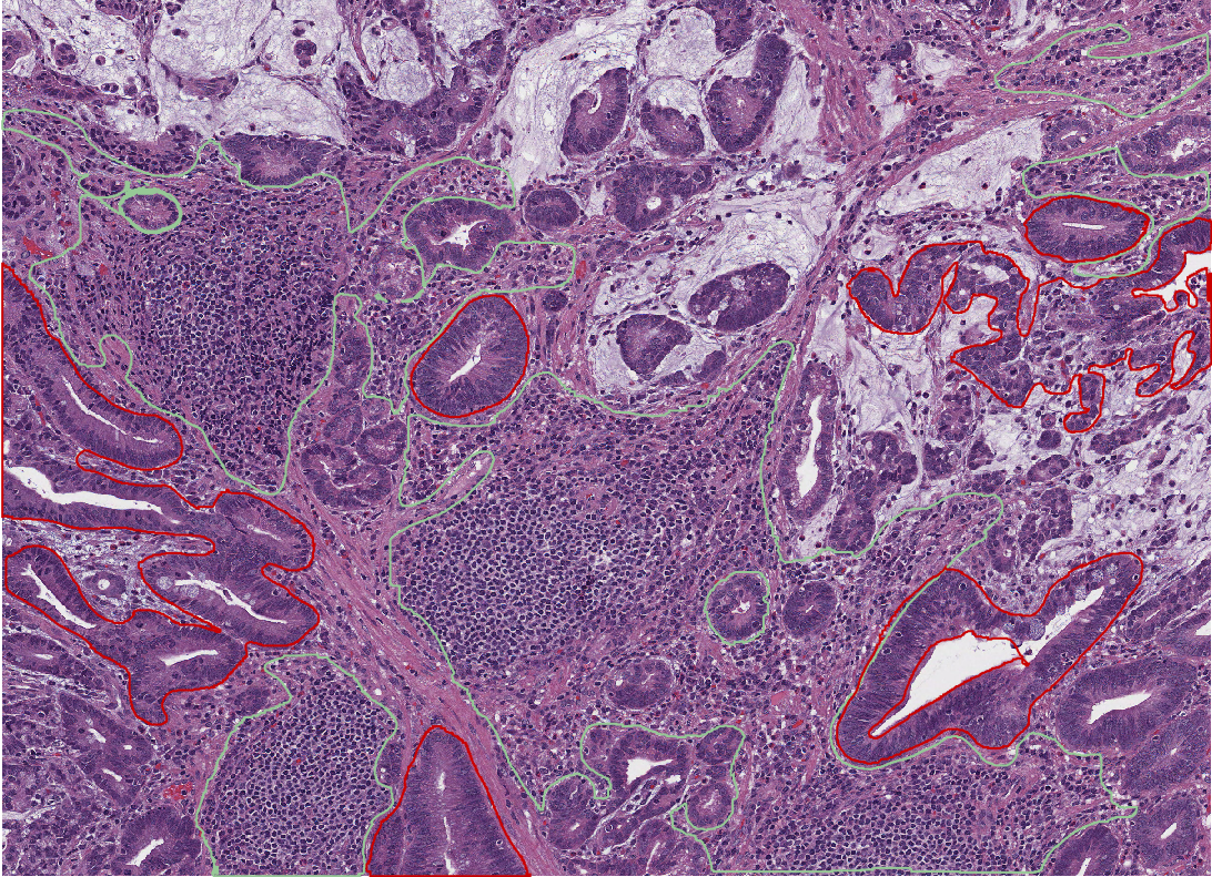
Fig. 2.16 – The annotations are classified as tumor or stroma.

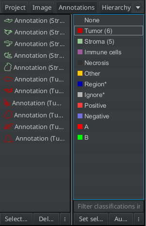
Fig. 2.17 – Annotations can be classified from the class list widget of the Annotations-tab.

You can classfiy the selected annotations by selecting a class in the class-list and pressing the Set-selected-button or view the Set classification-menu of the viewer's context menu. When Auto set is selected on the class-list widget, the new annotations you create will have the selected class.

To select the objects of a given class, use the menu Objects>Select>Select objects by classification or call the command from the context menu of a class in the class-list.

Note

Note that you find the class of an annotation in the measurements of the annotation object and the class in the class list tells you how many annotations of a given class are in the image. However you do not find the number of objects of a given class in the summary-measurements as is the case with detections.

2.2.9 Annotations vs. Detections

Annotations and detections both represent objects in QuPath. The main difference is that annotations can be modified after their creation and detections can not. Furthermore Annotations can be the parents of other objects, while detections can only be the children. Detections should be used when a great number of objects is created while annotations are rather used for a limited number objects.

Annotations	Detections
a region of interest	an object, for example a cell
limited number	large number
has a name and a description	no name or description
can have a class	can have a class
has measurements	has measurements
can be parent in a hierarchy	can not be parent in a hierachy
can be child in a hierarchy	can be child in a hierarchy
can be modified	can not be modified

Table 2.1 – Comparison of annotations and detections.

You can convert annotations into detections and vice versa, using a script. To execuite one of the script below, open the script editor from Automate>Script editor, copy the script into the editor and execute the Run command from the editor's Run-menu. Before running the script, you need to select the annotations or detections you want to convert.

Script 2.1 – Convert selected annotations to detections.

def annotations = getSelectedObjects().findAll {
    it.isAnnotation() && it.getChildObjects().isEmpty() 
}
def detections = annotations.each {
    detection = new qupath.lib.objects.PathDetectionObject(it.getROI(), it.getPathClass())
    parent = it.getParent()
    if (parent.isAnnotation()) {
        parent.addChildObject(detection)
    }
}
removeObjects(annotations, true)

Script 2.2 – Convert selected detections to annotations.

def detections = getSelectedObjects().findAll {
   it.isDetection() 
}
def annotations = detections.each {
    annotation = new qupath.lib.objects.PathAnnotationObject(it.getROI(), it.getPathClass())
    parent = it.getParent()
    if (parent.isAnnotation()) {
        parent.addChildObject(annotation)
    }
}
removeObjects(detections, true)

2.3 Measurements

To see the measurements of an annotation, look at the lower part of the annotations tab. The overall number of detections within the annotation is shown as well as the number of detections per class if the detections have been classified. By default the centroid, the perimeter and the area of the annotation are measured. Other shape and intensity measurements can be added.

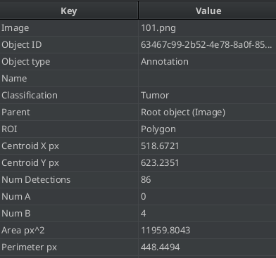
Fig. 2.18 – Measurements of the selected annotation.

The measurements are also called features, since the can be used to train machine learning classifiers. The submenus Add Intensity Features and Add Shape Featues of the menu Analyze>Calculate Features allow to add selected measurements.

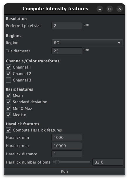
Fig. 2.19 – Add intensity measurements on different channels.

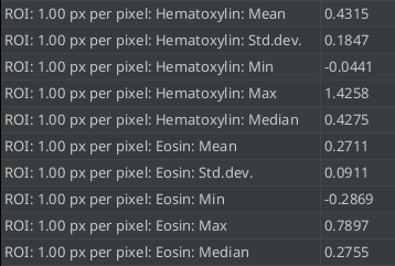
Fig. 2.20 – Intensity measurements on different channels.

Red, Green and Blue are the channels of the usual rgb-colour model. Hue, saturation and brightness are the channels of the HSB color model. Optical density and color deconvolution are the topic of chapter 3. Haralick features [1] also known under the name Gray Level Co-occurrence Matrices (GLCM), describe the texture of a region based on the spatial dependencies of pixel intensities.

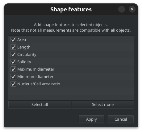
Fig. 2.21 – Adding shape features.

The circularity is defined by formula 2.1. It is a value between 0 and 1. The circularity of a circle is 1, the circularity of a square is approximatly 0.8 and the circularity of a rectangle that is two times larger than wide is about 0.7

$$ c = 4 \pi \cdot \frac{area}{(perimeter)²} \tag{2-1} $$

The solidity, is the ratio of the area of the annotation and its convex area, i.e. its area when holes and concavities are removed.

$$ s = \frac{area}{convex\ area} \tag{2-2} $$

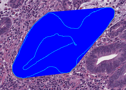
Fig. 2.22 – The area is marked by the light blue contour and the convex area by the region filled in dark blue.

Measurements on all annotations of an image can be displayed and exported via the menu Measure>Show Annotation Measurements. The table can be sorted by a given column and a click on a row also selects the annotation in the image. The other way round, selecting an annotation in the image also selects its row in the table when the table is open. Histograms and scatter plots can be created from the widget and the measurements can saved to a tab-separated text file, that you can open with your favorite spreadsheet software.

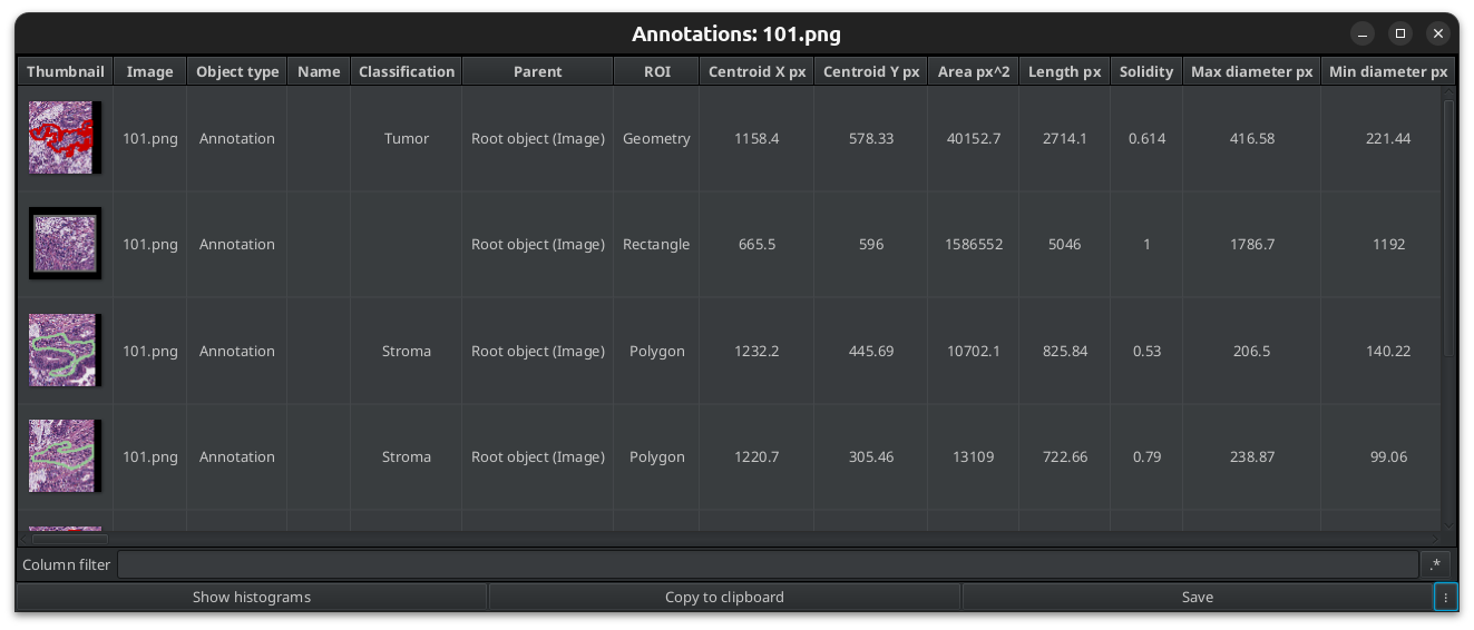
Fig. 2.23 – Annotation Measurements of the annotations in the current image.

Finally the measurements of all objects of all images in the project can be exported via the menu Measure>Export Measurements.... To export annotations, select the export type Annotations. You can press the Populate button, select the columns od interest and export only the selected columns if you do not want to export all measurements.

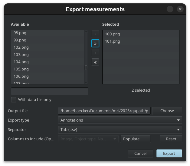
Fig. 2.24 – Export the measurements from objects on multiple images.

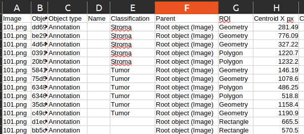
Fig. 2.25 – The exported measurements as a spreadsheet.

Literature

1. Haralick, R.M., Shanmugam, K., Dinstein, I., 1973. Textural Features for Image Classification. IEEE Trans. Syst., Man, Cybern. SMC-3, 610–621.